Stereo Visual Odometry
Brief overview
Visual odometry is the process of determining the position and orientation of a mobile robot by using camera images. A stereo camera setup and KITTI grayscale odometry dataset are used in this project. KITTI dataset is one of the most popular datasets and benchmarks for testing visual odometry algorithms. This project aims to use OpenCV functions and apply basic cv principles to process the stereo camera images and build visual odometry using the KITTI dataset.
Video demo
Algorithm descriptions
KITTI dataset:
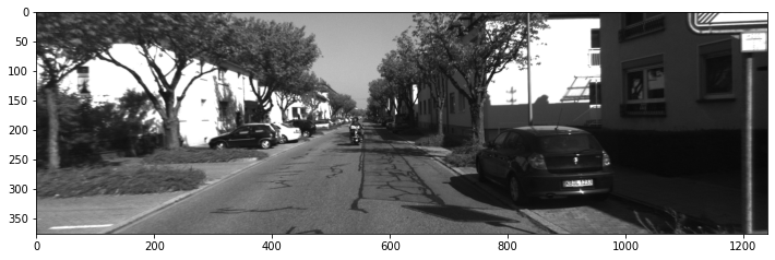
KITTI is a real-world computer vision datasets that focus on various tasks, including stereo, optical flow, visual odometry, 3D object detection, and 3D tracking. In this project, only the visual odometry data will be used. For this task, only grayscale odometry data set and odometry ground-truth poses are needed. The grayscale image is used as the input image. The ground-truth poses are used to compare with the pose generated by the algorithm. Figure 1 shows the first grayscale frame of the left camera from the data set. More information about the sensor setup can be found here.
Data processing:
The data is processed in the “Dataset_Handler” class. The class can store the image data and easily extract and use both image and sensor calibration data. Since the one folder of images will take around 30GB of RAM if stored as a list, a generator stores one frame of the image each time we call the function.
Calibration data:
The calibration information can be found in the data set for each of the two cameras. The calibration data can be extracted in the form of the projection matrix. The projection matrix is a 3 by 4 matrix which contains information about a 3 by 3 intrinsic matrix of the camera, a 3 by 3 rotation matrix, and a 3 by 1 translation matrix of the camera pose.
Depth calculation:
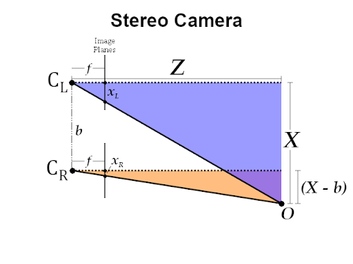
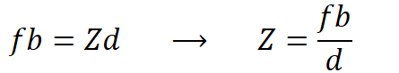
In theory, it is difficult to obtain the depth information from a single pinhole camera; however, it is possible using a stereo camera setup. In Figure 2, a schematic shows one target pixel projected in two image planes. We can solve for depth using similar triangles, as shown in Figure 3. In the equation, z is the depth of the pixel in meters, f is the focal length in the x-direction in pixels, b is the baseline distance between the two cameras which is 0.54m, and d is the disparity between the same points between the two images in pixels. We already know the camera’s focal length and baseline distance to calculate the depth. We still need to find the disparity between the left and right frame, described in the next section.
Disparity calculation:
The disparity describes the difference between the same pixel projected to two separated cameras. There are a few ways of stereo matching available in OpenCV to find disparity. The two methods tested in the project are stereo block-matching (StereoBM) and stereo semi-global block-matching (StereoSGBM). Figure 4 below shows the disparity map using the stereo block-matching method, while Figure 5 shows the disparity map using the stereo semi-global block-matching.
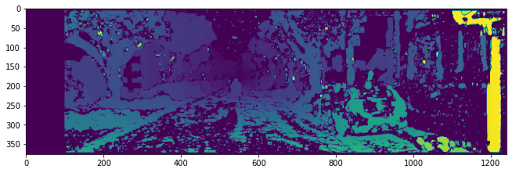
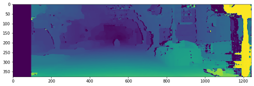
The darker color indicates smaller disparity; however, the darkest color in the map (purple) indicates the regions that the matching method could not successfully detect. It is noticeable that there is one column on the left that the algorithm could not match, which makes sense because the two cameras are separated by a distance which will then cause a shift from the left camera to the right camera when recording images. Comparing the disparity maps rendered from the two methods, it is easy to tell that the semi-global block-matching method results in a smoother image with fewer dark gaps in the frame. However, the blocking-matching method only takes around 42 ms to process a frame, while the semi-global blocking-matching method takes 99 ms.
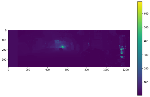
After calculating out the disparity map, we are ready to calculate the depth of the frame based on the depth formula provided in the previous section. Figure 6 shows the depth map after the calculation. The yellow pixels are the furthest regions, while the purple ones are the closest. The map is reasonable since the furthest region is the center of the image in the first frame, matching the original image.
Feature extraction and match:
In order to find and generate a path, we would need to find some key features and keep track of them. Those key features would be found between the current frame of the left camera and the next frame of the same camera. SIFT by David Lowe is a classic and robust feature extracting approach which computes the scale and rotation invariant feature descriptor. Another approach called ORB is also used as a comparison.
In this project, a Brute-Force matching algorithm is used to match all the features extracted previously. The algorithm takes the descriptor from the matching features of the current frame and is matched with all other features in the next frame using some distance calculation, and then chooses the closest one to match with.
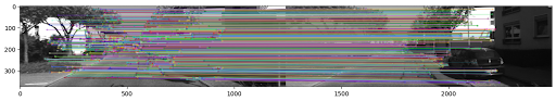
Figures 7 and 8 show the two matching results using different feature extraction methods (SIFT and ORB). Moreover, they are both matched using Brute-Force. For SIFT algorithm, there are 2931 features found in total. It took around 100 ms for each of the two images to extract features and around 266 ms to match the features from the two frames. For the ORB algorithm, there are 500 features found in total. It took around 30 ms for each of the two images to extract features and around 70 ms to match the features from the two frames.
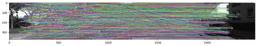
SIFT approach has a better performance which detects five times more than the features extracted by ORB. However, the ORB approach is approximately three times faster than SIFT regarding the processing time. For both methods, especially the SIFT methods, we can find some matching lines that are not horizontal, which are wrong since the feature detected would not move too much in the y-direction from frame to frame. Then a method was proposed by David Lowe to filter out some outliers. A ratio test was implemented to determine the level of distinctiveness of features. The test compares the ratios of the distance of two matched descriptors and generates a probability density function for correct and incorrect matches based on the ratio of distances. Figure 9 shows the plot of the probability density function.
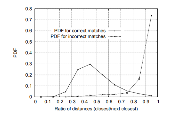
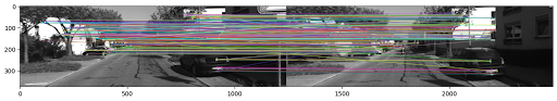
From the plot, we can conclude that the closer the two distances of the two matches are, the less likely they are correct matches. Also, the chance of correct matches hits a peak when at a ratio of distances of around 0.45. Therefore, a threshold of 0.45 was set in the project to filter out matches with ratios of distances higher than 0.45. After the low pass filter, the matches drop to 826 for SIFT approach and to 75 for the ORB approach. Figure 10 shows the matching map using SIFT method after the low pass filter. The matching lines are all nearly horizontal after the filter.
Motion estimation:
This section needs to solve for a rotation matrix and a translation vector for each frame. The PnP algorithm with RANSAC is an effective solver handling outliers well. The PnP solver takes a list of 1 by 3 vectors of 3D coordinates in meters from the current frame, a list of 1 by 2 vectors of 2D coordinates in pixels from the next frame, the intrinsic matrix of the camera, and then solve for the rotational matrix and translation vector of that frame. RANSAC minimizes the reprojection error and makes this function robust to outliers.
Visual odometry (main function):
In this section, the main function will be constructed, which calls the previously made functions to generate a trajectory based on the pose of each frame. For each iteration, a pair of subsequent frames are input to the PnP RANSAC solver, and then a pose consists of both rotation and translation matrix will be returned. A 4 by 4 homogenous transformation matrix will be constructed based on those two matrices. The transformation matrix calculated transforms the current frame to the next frame. We have to inverse the matrix and then multiply the previous transformation matrix to transform the next frame to the world frame. The world frame is the initial pose of the camera. The previous transformation matrix is an identity matrix for the first iteration and then accumulates for the rest iteration. Every pose of each iteration is then stored in a trajectory list and later used in plotting the estimated path.
Results
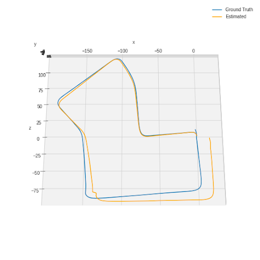
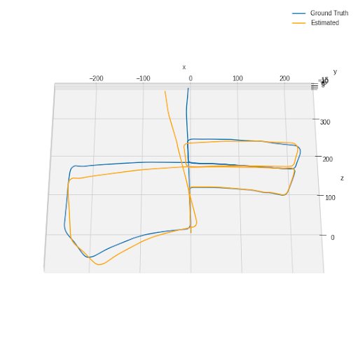
Figure 11 shows the resultant plot of the estimated path and ground-truth path for scene 7 of the dataset. The ground Truth path is plotted as a blue line, and the estimated path is the yellow line. From the view of the left camera at the first frame, the positive z-direction is forward, positive y-direction is downward, and positive is rightward. After generating the trajectory of the estimated path, a calculation was implemented to calculate the distance between the endpoint of the ground-truth path and the estimated path. The distance is calculated to be 24.18 m for scene 7. Figure 12 shows the plot of both ground truth and estimated path using odometry data from scene 5. The distance between the endpoints of the ground truth and the estimated path is calculated to be 50.12 m.